Data
As in previous documents, we have imported the data such as it was at the end of analysis_02, and it is now loaded and available as df_long and df_wide.
Tense~lax mergers before /l/
The relevant pairs - FLEECE-KIT, FACE-DRESS, and GOOSE-FOOT, all preceding /l/ - are so rare that I would venture we shouldn’t include them in the global datasets.
The onset of FACE
Speaker-level
For this feature, we can conduct the speaker-level analysis by simply asking: who has the lowest FACE centroid at 20%, i.e. the highest F1 value?
df_long %>%
  filter(timepoint == 20,
         vowel == "FACE") %>%
  group_by(name) %>%
  summarise(face_onset = mean(f1_lobanov),
            dataset = nth(dataset, 1)) %>%
  mutate(face_onset = (face_onset + 1.1)) %>%
  #-----viz-----#
  ggplot(aes(x = reorder(name, face_onset),
             y = face_onset,
             fill = dataset)) +
  geom_col(stat = "identity",
           width = 0.5)          +
  scale_fill_grey(start = 0,
                  end = 0.8)     +
  coord_flip()                   +
  labs(
    title = "Lowering of the FACE onset",
    x = NULL,
    y = "normalized F1 at 20% duration") +
  theme_classic(base_family = "Roboto Condensed")
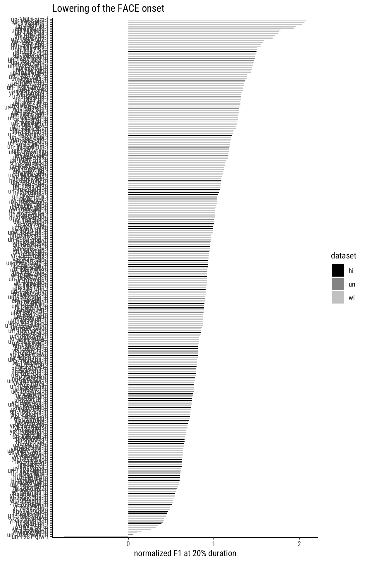
The darker shades here, as per the legend, are for the newer datasets. And while the tendency is not overwhelmingly clear, one could say that the higher F1-values are more clearly provided by bars in the lightest shade, i.e. by the older speakers.
Token-level
We’ll append F1 at 20% to a dedicated col. called face_lowering in df_wide for all rows where vowel == "FACE".
df_wide <- df_wide %>%
  mutate(face_lowering =
           ifelse(vowel == "FACE", f1_lobanov_20, NA))
MOUTH fronting
This feature is a very clear marker of southernness. Very conservative. It lies in the frontness of F2 at 20%.
Speaker-level
df_long %>%
  filter(timepoint == 20,
         vowel == "MOUTH") %>%
  group_by(name) %>%
  summarise(mouth_fronting = mean(f2_lobanov),
            dataset = nth(dataset, 1)) %>%
  mutate(mouth_fronting = (mouth_fronting + 0.9)) %>%
  #-----viz-----#
  ggplot(aes(x = reorder(name, mouth_fronting),
             y = mouth_fronting,
             fill = dataset)) +
  geom_col(stat = "identity",
           width = 0.5)          +
  scale_fill_grey(start = 0,
                  end = 0.8)     +
  coord_flip()                   +
  labs(
    title = "Fronting of MOUTH",
    x = NULL,
    y = "normalized F2 at 20% duration") +
  theme_classic(base_family = "Roboto Condensed")

You can call me a simpleton if you like, but I think this picture looks very similar to the one for FACE lowering above.
Token-level
Let’s add the value for F2 at 20% to the right of df_wide for all rows where vowel == MOUTH.
df_wide <- df_wide %>%
  mutate(mouth_fronting =
           ifelse(vowel == "MOUTH", f2_lobanov_20, NA))
LOT~THOUGHT Merger
Narrowing down the LOT class
DARLA distinguishes between THOUGHT and other low-back vowels, but those are all rolled together… which is why we have a class “LOT/PALM/START”. In order to really study the LOT~THOUGHT phenomenology in an epistemologically sound way, let’s run some exclusions.
- No LOT/PALM/START vowels with following /r/, because those are the words in the START class.
- No LOT/PALM/START with the orthographic sequence
, which describes the PALM words. - Nor any
or sequences, as they tend to occur in THOUGHT, not in LOT. - No word-final to exclude words like bra, spa.
- Exclude father, lager.
- Exclude a number of misspelled tokens that struck me during optical inspection of the list.
Running those exclusions, we end up with the following members of the LOT/PALM/START class.
lotwords <-
  df_long %>%
  filter(timepoint == 50,
         vowel == "LOT/PALM/START",
         !fol_seg %in% c("R", "L"),
         # lexical exclusions
         !word %in% c("FATHER", "FATHER'S",
         "FATHERS", "LAGER", "MAH", "LAS",
         "MILAN"),
         # misspellings
         !word %in% c("",
                      "WAH", "WAS",
                      "WASN'T", "WASN'TT",
                      "FATEHR"),
         !str_detect(word, "AU"),
         !str_detect(word, "AL"),
         !str_detect(word, "A$")
         ) %>%
  count(word)

lotwords %>%
  kbl() %>%
  kable_paper("striped")
| word | n |
|---|---|
| ACCOMPLISHED | 1 |
| ACCOMPLISHMENTS | 1 |
| ADOPTED | 1 |
| ADOPTING | 1 |
| ADOPTS | 1 |
| AWE | 2 |
| AWFUL | 7 |
| AWFULLY | 1 |
| BACL | 1 |
| BEYOND | 15 |
| BLAH | 5 |
| BLOCK | 13 |
| BLOCKED | 2 |
| BLOCKS | 3 |
| BLOCKSTREET | 2 |
| BLOKS | 1 |
| BODIES | 1 |
| BODY | 1 |
| BODY’S | 1 |
| BOGS | 4 |
| BOMB | 44 |
| BOND | 2 |
| BONDING | 3 |
| BONDNESS | 1 |
| BOSS | 1 |
| BOTHER | 63 |
| BOTHERED | 1 |
| BOTHERING | 1 |
| BOTHERS | 2 |
| BOTTLE | 6 |
| BOTTOM | 4 |
| BOX | 1 |
| CHAVEZ | 3 |
| CHICAGO | 2 |
| CHICANO | 1 |
| CHOPPY | 1 |
| CHOREOGRAPHY | 1 |
| CLOCK | 1 |
| CLOSET | 6 |
| COB | 2 |
| COBS | 54 |
| COCK | 47 |
| COFFEE | 1 |
| COLORADO | 4 |
| COM | 2 |
| COMMENTS | 1 |
| COMMON | 17 |
| COMMONS | 1 |
| COMMUNE | 4 |
| COMMUNISM | 1 |
| COMMUNIST | 1 |
| COMPLEX | 2 |
| COMPLEXES | 2 |
| COMPLICATED | 7 |
| CONCEPT | 1 |
| CONDOS | 1 |
| CONFIDENCE | 2 |
| CONFIDENT | 6 |
| CONFLICT | 1 |
| CONGRESS | 8 |
| CONGRESSMEN | 1 |
| CONNELY | 1 |
| CONRETE | 1 |
| CONSTANT | 3 |
| CONTEXT | 1 |
| CONTROVERSIES | 1 |
| COOPERATIVES | 1 |
| COP | 3 |
| COPS | 1 |
| CORRESPONDENCE | 3 |
| COST | 5 |
| COT | 49 |
| COTTAGE | 2 |
| COTTON | 1 |
| CROCKETT | 1 |
| CROP | 3 |
| CROPS | 1 |
| DOCTOR | 1 |
| DOCTOR’S | 4 |
| DOCTORATE | 1 |
| DOD | 1 |
| DOGGET | 1 |
| DOGS | 60 |
| DON | 41 |
| DONKEY | 47 |
| DONT | 2 |
| DONW | 1 |
| DOT | 1 |
| DROP | 57 |
| DROPPED | 5 |
| DROPPING | 1 |
| DROPS | 14 |
| ECONOMIC | 6 |
| ECONOMY | 11 |
| ECONOMY’S | 1 |
| FOG | 4 |
| FOGGY | 49 |
| FONTS | 2 |
| FORGOT | 1 |
| FOSTER | 1 |
| FROG | 5 |
| FROGS | 3 |
| GAH | 1 |
| GARAGE | 9 |
| GEOGRAPHY | 1 |
| GOD | 10 |
| GODS | 13 |
| GOSSIP | 1 |
| GOT | 7 |
| GROVEL | 4 |
| HAH’D | 13 |
| HOBBY | 1 |
| HOCK | 48 |
| HOD | 240 |
| HOG | 2 |
| HOMOGENOUS | 1 |
| HONEST | 6 |
| HONESTLY | 1 |
| HOPPIN | 40 |
| HOPPING | 16 |
| HOSTILE | 1 |
| HOT | 13 |
| JOB | 143 |
| JOBS | 11 |
| JOG | 1 |
| JOHN | 56 |
| JOHNS | 3 |
| JOHNSON | 4 |
| JOHNSTON | 3 |
| JOPLIN | 1 |
| KNOCK | 2 |
| KNOCKED | 1 |
| LOBBY | 1 |
| LOCK | 3 |
| LOCKING | 1 |
| LOT | 237 |
| LOTS | 74 |
| MASSAGE | 1 |
| MODERATE | 5 |
| MODERATELY | 522 |
| MODERATLEY | 1 |
| MODERN | 3 |
| MODEST | 2 |
| MOM | 22 |
| MOM’S | 6 |
| MOMS | 1 |
| MONOTONY | 1 |
| NON | 11 |
| NOT | 17 |
| NOTCH | 1 |
| O’CLOCK | 5 |
| OBJECT | 1 |
| OBJECTS | 1 |
| OBVIOUS | 1 |
| OBVIOUSLY | 3 |
| ODD | 52 |
| ON | 10 |
| OP | 1 |
| OPPERATOR | 1 |
| OPPERTUNITY | 2 |
| OPPOSITE | 2 |
| OPTION | 2 |
| PATRIOTIC | 1 |
| PECAN | 46 |
| PHENOMENON | 2 |
| PHILOSOPHY | 3 |
| PHOTOGRAPHY | 43 |
| PLODDED | 2 |
| 4 | |
| PONDS | 3 |
| POP | 106 |
| POPCORN | 101 |
| POPERTY | 1 |
| POPPED | 2 |
| POPULAR | 1 |
| POSITIVE | 5 |
| POSSIBLE | 4 |
| POSSIBLY | 2 |
| POSSUMS | 4 |
| POT | 15 |
| POTTY | 2 |
| POVERTY | 1 |
| PRAGUE | 1 |
| PREDOMINANTLY | 1 |
| PREDOMINATELY | 1 |
| PROBABLY | 103 |
| PROBLEM | 9 |
| PROBLEMS | 14 |
| PROCESS | 4 |
| PROCESSED | 2 |
| PRODUCT | 5 |
| PRODUCTS | 2 |
| PROFITABLE | 1 |
| PROGRESS | 106 |
| PROJECT | 3 |
| PROJECTS | 2 |
| PROPER | 1 |
| PROPERLY | 1 |
| PROPERTIES | 1 |
| PROPERTY | 24 |
| PROPERY | 1 |
| PROPSING | 1 |
| PROSECUTED | 1 |
| REMODELED | 1 |
| ROBBLE | 1 |
| ROBERT | 2 |
| ROBOT | 1 |
| ROCK | 6 |
| ROCKS | 3 |
| RODDENBERRY | 1 |
| RODS | 4 |
| ROSS | 2 |
| ROT | 45 |
| ROTC | 2 |
| ROTTED | 2 |
| ROTTEN | 59 |
| SCOTT | 1 |
| SHOCK | 2 |
| SHOP | 3 |
| SHOPPING | 1 |
| SHOT | 9 |
| SHOTS | 2 |
| SLOT | 1 |
| SNOBBISH | 1 |
| SOCCER | 3 |
| SOD | 46 |
| SOFT | 1 |
| SPONSERS | 1 |
| SPOTS | 1 |
| SQUATTED | 3 |
| STOC | 1 |
| STOCK | 56 |
| STOP | 62 |
| STOPPED | 3 |
| TOD | 1 |
| TOM | 2 |
| TOMAS | 3 |
| TOMAS’S | 1 |
| TOMMY | 1 |
| TOP | 7 |
| TOPOGRAPHY | 1 |
| TRODDED | 1 |
| TROTTED | 1 |
| UNGODLY | 1 |
| UPON | 19 |
| WANT | 54 |
| WANTS | 2 |
| WASH | 4 |
| WASHINGTON | 16 |
| WATCH | 11 |
| WATCHED | 60 |
| WATCHING | 7 |
So those are our LOT-words. I’ll place them in a vector and use that to filter out the rows of interest for the LOT~THOUGHT analysis.
lotwords <- lotwords %>%
  pull(word)
lotwords %>% str()
chr [1:252] "ACCOMPLISHED" "ACCOMPLISHMENTS" "ADOPTED" ...Define the dataset
Speaker-level
Get speaker-level scores
speakers <- df_long %>%
  pull(name) %>%
  unique()

pillai_lotthought <- tibble()
wins <- c()
fails <- c()

for (s in (1:length(speakers))){
  # cat("\nspeaker no. ", s)
  dat_s <- dat %>%
    filter(name == speakers[s]) %>%
    mutate(f1_lobanov =
           as.numeric(f1_lobanov),
           f2_lobanov =
           as.numeric(f2_lobanov))

  v1 <- unique(dat_s$vowel)[1]
  n_v1 <- dat_s %>% filter(vowel == v1) %>% nrow()
  if (n_v1 < 6) next

  v2 <- unique(dat_s$vowel)[2]
  n_v2 <- dat_s %>% filter(vowel == v2) %>% nrow()
  if (n_v2 < 6) next

  if (length(unique(dat_s$vowel)) == 2 &
      length(unique(dat_s$vowel))) {
      my_man <- manova(cbind(f1_lobanov,
                             f2_lobanov) ~ vowel,
                       data = dat_s)
      pil <- summary(my_man, tol=0)$stats["vowel",
                                   "Pillai"]
      # wins <- append(wins, s)
      # n_success <- length(wins)
      # cat("\nsuccess", n_success, ":",
      #     s, ":",
      #     pil)

  } else {
    # fails <- append(fails, s)
    # cat("\nfail", length(fails), ":",
    #     s)
    next
    }

  newscore <- tibble(name = speakers[s],
                     lotthought_pillai = pil)

  pillai_lotthought <-
    bind_rows(pillai_lotthought, newscore) %>%
    arrange(desc(lotthought_pillai)) %>%
    unique()
}

pillai_lotthought
# A tibble: 160 x 2
name lotthought_pillai
<chr> <dbl>
1 un-1987-dcl-f 0.885
2 un-1987-jak-m 0.811
3 un-1987-wyf-m 0.763
4 un-1987-gb-m 0.743
5 un-1987-ffw-f 0.739
6 un-1987-aam-m 0.716
7 un-1987-hcb-m 0.692
8 un-1987-dr2-f 0.677
9 un-1987-blb-m 0.672
10 un-1987-is-f 0.666
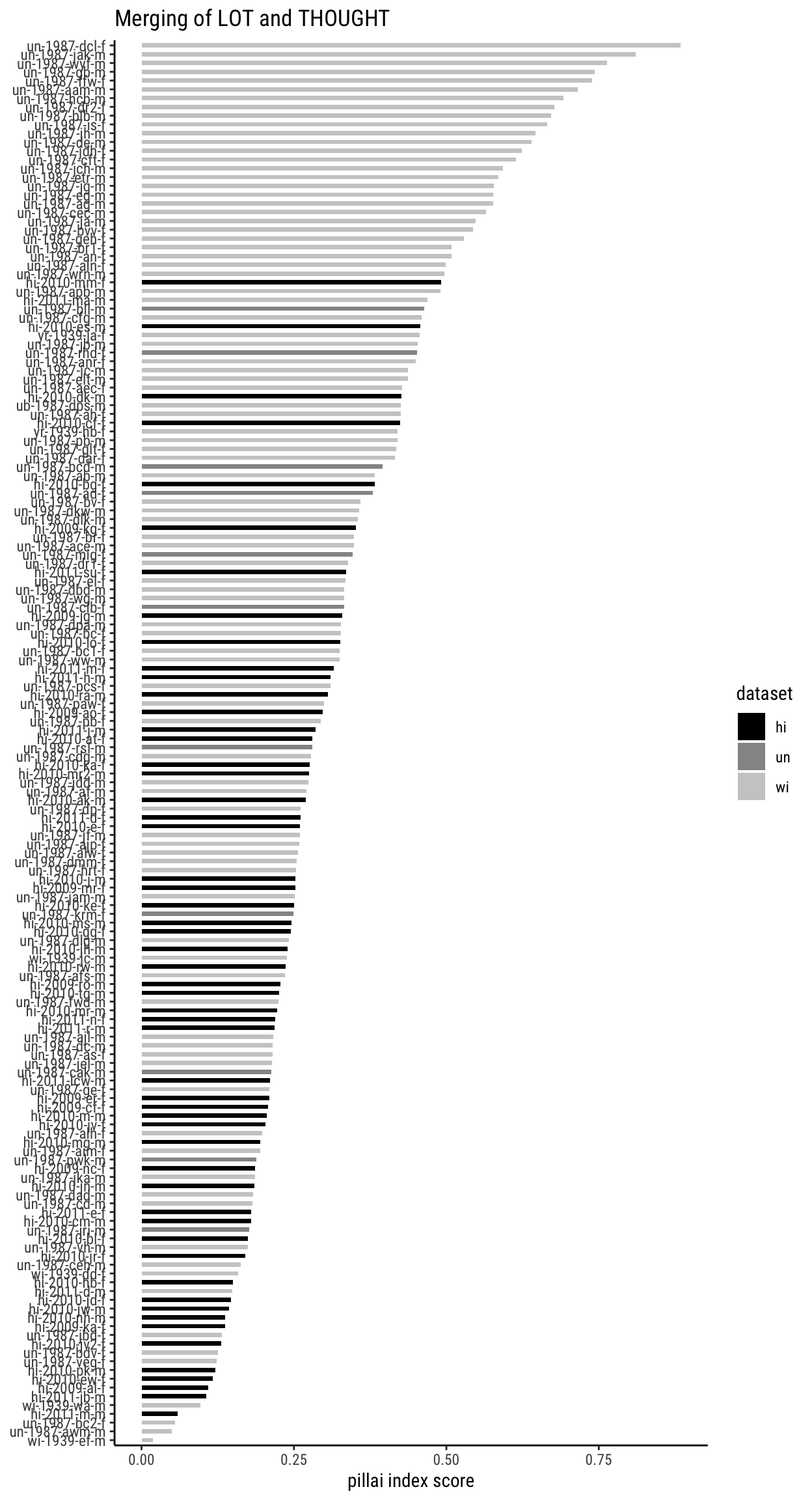
# … with 150 more rowsVisualize speaker-level scores
datas <- df_long %>%
  group_by(name) %>%
  summarise(dataset = nth(dataset, 1)) %>%
  select(name, dataset)

pillai_lotthought %>%
  left_join(datas) %>%
  ggplot(aes(x = reorder(name, lotthought_pillai),
             y = lotthought_pillai,
             fill = dataset))    +
  geom_col(stat = "identity",
           width = 0.5)          +
  scale_fill_grey(start = 0,
                  end = 0.8)     +
  coord_flip()                   +
  labs(
    title = "Merging of LOT and THOUGHT",
    x = NULL,
    y = "pillai index score") +
  theme_classic(base_family = "Roboto Condensed")
Token-level
We’ll add the distance of each LOT or THOUGHT token from the centroid of the OTHER vowel to two to-be-created columns at the right of df_wide.
Obtain LOT and THOUGHT centroids for each speaker
# define speakers again, this time with dataset
speakers <- df_long %>%
  select(name, dataset) %>%
  unique()

# make empty results obj for all speakers
lot_and_thoughts <- tibble()

# get results
for (s in (1:nrow(speakers))){

  # get speaker-level info
  speaker <- speakers %>%
    pull(name) %>%
    nth(s)
  dataset <- speakers %>%
    pull(dataset) %>%
    nth(s)

  # get LOT centroid
  lot_s <- dat %>%
    getspeakervowel(speaker, "LOT")  %>%
    unlist()

  # get THOUGHT centroid
  thought_s <- dat %>%
    getspeakervowel(speaker, "THOUGHT")  %>%
    unlist()

  results_s <-
    c(speaker, dataset, lot_s, thought_s)

  names(results_s) <- c("name", "dataset",
                        "f1_lot", "f2_lot",
                        "f1_thought", "f2_thought")

  # append speaker results to results
  lot_and_thoughts <- bind_rows(lot_and_thoughts,
                                results_s) %>%
    na.omit()
}

(lot_and_thoughts <-
  lot_and_thoughts %>%
  mutate(across(starts_with("f"), as.numeric)))
# A tibble: 290 x 6
   name         dataset f1_lot f2_lot f1_thought f2_thought
   <chr>        <chr>    <dbl>  <dbl>      <dbl>      <dbl>
 1 hi-2009-ab-f hi       0.899 -0.754      0.833      -1.34
 2 hi-2009-al-f hi       1.15  -0.860      0.735      -1.13
 3 hi-2009-cf-f hi       1.15  -0.962      0.445      -1.30
 4 hi-2009-er-f hi       0.832 -0.730      0.494      -1.11
 5 hi-2009-jg-m hi       1.27  -0.915      0.362      -1.42
 6 hi-2009-kg-f hi       1.00  -0.906      0.198      -1.49
 7 hi-2009-mr-f hi       1.11  -0.874      0.389      -1.37
 8 hi-2009-nc-f hi       1.07  -0.928      0.209      -1.27
 9 hi-2009-ro-m hi       1.26  -0.917      0.448      -1.33
10 hi-2010-ak-m hi       1.01  -0.886      0.455      -1.34
# … with 280 more rows
Get token-level distance measure and attach to df_wide
Get the token-level distance measure.
The distance measures are now contained in dat. We’ll reduce it to only the columns vowelID, ed_from_lot and ed_from_thought. And then join it with df_wide.
dat <-
  dat %>%
  select(vowelID, ed_from_lot, ed_from_thought)

df_wide <-
  df_wide %>%
  left_join(dat)
Save data
Save the data sheets. Include suffix _03 in the filename to indicate that this version of the data is produced by the document analysis_03.Rmd.
df_long %>% export("../../_data/data_long_03.RDS")
df_wide %>% export("../../_data/data_wide_03.RDS")