Data
We start out with a long-version dataset, df_long:
df_long %>% glimpse()
Rows: 457,475
Columns: 30
$ vowelID      <int> 1, 1, 1, 1, 1, 2, 2, 2, 2, 2, 3, 3, 3, 3, 3, 4…
$ name         <chr> "hi-2009-ab-f", "hi-2009-ab-f", "hi-2009-ab-f"…
$ vowel        <chr> "DRESS", "DRESS", "DRESS", "DRESS", "DRESS", "…
$ word         <chr> "YES", "YES", "YES", "YES", "YES", "TWENTY", "…
$ style        <chr> "interview", "interview", "interview", "interv…
$ timepoint    <int> 20, 35, 50, 65, 80, 20, 35, 50, 65, 80, 20, 35…
$ f1_hz        <dbl> 680.5, 1061.8, 810.7, 836.8, 998.3, 656.1, 609…
$ f2_hz        <dbl> 2203.0, 1810.9, 1836.9, 1876.5, 2002.8, 1497.9…
$ f1_lobanov   <dbl> 0.01943932, 2.35367923, 0.81649685, 0.97627566…
$ f2_lobanov   <dbl> 1.1975892, 0.1243169, 0.1954852, 0.3038799, 0.…
$ dur          <dbl> 0.23, 0.23, 0.23, 0.23, 0.23, 0.17, 0.17, 0.17…
$ plt_vclass   <chr> "e", "e", "e", "e", "e", "e", "e", "e", "e", "…
$ plt_manner   <chr> "fricative", "fricative", "fricative", "fricat…
$ plt_place    <chr> "apical", "apical", "apical", "apical", "apica…
$ plt_voice    <chr> "voiceless", "voiceless", "voiceless", "voicel…
$ plt_preseg   <chr> "w/y", "w/y", "w/y", "w/y", "w/y", "w/y", "w/y…
$ plt_folseq   <chr> "", "", "", "", "", "complex_one_syl", "comple…
$ pre_seg      <chr> "Y", "Y", "Y", "Y", "Y", "W", "W", "W", "W", "…
$ fol_seg      <chr> "S", "S", "S", "S", "S", "N", "N", "N", "N", "…
$ context      <chr> "internal", "internal", "internal", "internal"…
$ dataset      <chr> "hi", "hi", "hi", "hi", "hi", "hi", "hi", "hi"…
$ yearRecorded <int> 2009, 2009, 2009, 2009, 2009, 2009, 2009, 2009…
$ initials     <chr> "ab", "ab", "ab", "ab", "ab", "ab", "ab", "ab"…
$ gender       <chr> "f", "f", "f", "f", "f", "f", "f", "f", "f", "…
$ yearBorn     <int> 1983, 1983, 1983, 1983, 1983, 1983, 1983, 1983…
$ ethnicity    <chr> "anglo", "anglo", "anglo", "anglo", "anglo", "…
$ townRaised   <chr> "austin", "austin", "austin", "austin", "austi…
$ occupation   <chr> "", "", "", "", "", "", "", "", "", "", "", ""…
$ beg          <dbl> 8.779, 8.779, 8.779, 8.779, 8.779, 13.496, 13.…
$ fileName     <chr> "../../../04 formant measurements (5 points DA…
as well as this wide-version dataset, df_wide:
df_wide %>% glimpse()
Rows: 91,495
Columns: 50
$ vowelID       <int> 1, 2, 3, 4, 5, 6, 7, 8, 9, 10, 11, 12, 13, 14…
$ name          <chr> "hi-2009-ab-f", "hi-2009-ab-f", "hi-2009-ab-f…
$ vowel         <chr> "DRESS", "DRESS", "KIT", "KIT", "STRUT", "PRI…
$ word          <chr> "YES", "TWENTY", "SIX", "PRETTY", "ADULT", "I…
$ style         <chr> "interview", "interview", "interview", "inter…
$ dur           <dbl> 0.23, 0.17, 0.29, 0.12, 0.05, 0.07, 0.05, 0.0…
$ plt_vclass    <chr> "e", "e", "i", "i", "uh", "ay", "o", "ow", "a…
$ plt_manner    <chr> "fricative", "nasal", "stop", "stop", "latera…
$ plt_place     <chr> "apical", "apical", "velar", "apical", "apica…
$ plt_voice     <chr> "voiceless", "voiced", "voiceless", "voiceles…
$ plt_preseg    <chr> "w/y", "w/y", "oral_apical", "obstruent_liqui…
$ plt_folseq    <chr> "", "complex_one_syl", "complex_coda", "one_f…
$ pre_seg       <chr> "Y", "W", "S", "R", "D", "", "G", "R", "M", "…
$ fol_seg       <chr> "S", "N", "K", "T", "L", "G", "T", "N", "W", …
$ context       <chr> "internal", "internal", "internal", "internal…
$ dataset       <chr> "hi", "hi", "hi", "hi", "hi", "hi", "hi", "hi…
$ yearRecorded  <int> 2009, 2009, 2009, 2009, 2009, 2009, 2009, 200…
$ initials      <chr> "ab", "ab", "ab", "ab", "ab", "ab", "ab", "ab…
$ gender        <chr> "f", "f", "f", "f", "f", "f", "f", "f", "f", …
$ yearBorn      <int> 1983, 1983, 1983, 1983, 1983, 1983, 1983, 198…
$ ethnicity     <chr> "anglo", "anglo", "anglo", "anglo", "anglo", …
$ townRaised    <chr> "austin", "austin", "austin", "austin", "aust…
$ occupation    <chr> "", "", "", "", "", "", "", "", "", "", "", "…
$ beg           <dbl> 8.779, 13.496, 13.886, 22.058, 22.558, 23.791…
$ fileName      <chr> "../../../04 formant measurements (5 points D…
$ f1_hz_20      <dbl> 680.5, 656.1, 595.5, 560.7, 584.6, 551.2, 704…
$ f1_hz_35      <dbl> 1061.8, 609.3, 564.9, 578.3, 584.6, 534.5, 70…
$ f1_hz_50      <dbl> 810.7, 624.8, 572.9, 564.8, 602.5, 680.8, 801…
$ f1_hz_65      <dbl> 836.8, 648.9, 516.9, 563.9, 601.9, 809.9, 871…
$ f1_hz_80      <dbl> 998.3, 608.0, 503.0, 556.9, 601.9, 742.7, 871…
$ f2_hz_20      <dbl> 2203.0, 1497.9, 1681.1, 1534.3, 1395.9, 1612.…
$ f2_hz_35      <dbl> 1810.9, 1846.3, 1556.3, 1548.1, 1395.9, 1615.…
$ f2_hz_50      <dbl> 1836.9, 1963.7, 1490.6, 1735.1, 1308.1, 1563.…
$ f2_hz_65      <dbl> 1876.5, 1479.1, 1553.8, 1693.1, 1232.7, 1850.…
$ f2_hz_80      <dbl> 2002.8, 1555.1, 1551.7, 1709.2, 1232.7, 1922.…
$ f1_lobanov_20 <dbl> 0.01943932, -0.12993245, -0.50091314, -0.7139…
$ f1_lobanov_35 <dbl> 2.35367923, -0.41643239, -0.68824003, -0.6062…
$ f1_lobanov_50 <dbl> 0.81649685, -0.32154459, -0.63926568, -0.6888…
$ f1_lobanov_65 <dbl> 0.976275663, -0.174009360, -0.982086120, -0.6…
$ f1_lobanov_80 <dbl> 1.9649453346, -0.4243907199, -1.0671790512, -…
$ f2_lobanov_20 <dbl> 1.19758924, -0.73243965, -0.23097703, -0.6328…
$ f2_lobanov_35 <dbl> 0.12431690, 0.22121524, -0.57258475, -0.59503…
$ f2_lobanov_50 <dbl> 0.1954852, 0.5425674, -0.7524215, -0.0831660,…
$ f2_lobanov_65 <dbl> 0.30387993, -0.78389978, -0.57942785, -0.1981…
$ f2_lobanov_80 <dbl> 0.64959352, -0.57586944, -0.58517606, -0.1540…
$ trajLN        <dbl> 5.3484379, 2.9910025, 1.0452673, 0.8092316, 0…
$ glideRaise    <dbl> -1.94550602, 0.29445827, 0.56626591, 0.023262…
$ glideFront    <dbl> -0.547995720, 0.156570206, -0.354199032, 0.47…
$ dist2080      <dbl> 2.0212108, 0.3334965, 0.6679177, 0.4793084, 0…
$ spectralRate  <dbl> 23.254078, 17.594133, 3.604370, 6.743597, 9.4…
Analyses
Prenasal TRAP/BATH raising
Prenasal raising index (PRI)
At the token level, what’s interesting to us is how far each prenasal token is removed from the speaker mean for the non-prenasal tokens. So this function takes the following steps:
- Go through data by speaker
- Determine speaker mean for non-prenasal TRAP/BATH
- New column: if a T/B token is prenasal, supply CD from speaker mean for non-prenasalT/B; otherwise NA
We start by extracting a dataframe with one entry for each speaker in the dataset, with their centroids for nonprenasal TRAP/BATH. Apologies - this move is quite slow! Might benefit from some tinkering later. This is some reduntant-ass code. But it works.
For now, I am going to set the following chunk to not run every time - we can run it manually one time, then the data will be written to disk, and imported from disk in the subsequent step.
#### Beginning of Axel's code
#nonprenasalTB <- df_long %>%
#     filter(! fol_seg %in% c("N", "M", "NG"),
#            timepoint==50,
#            vowel=="TRAP/BATH") %>%
#     group_by(name) %>%
#     summarize(f1lob_npntb = mean(f1_lobanov),
#               f2lob_npntb = mean(f2_lobanov))
#### End of Axel's code
# make a single-col dataframe of all speakers (i.e. 'name')
speakers <- df_long %>%
  select(name)      %>%
  unique()

# loop over main data by speaker and get
# centroid for non-prenasal TRAP/BATH (npntp);
# combine with speakers dataframe

# start python-style by setting empty container var
nonprenasalTB <- tibble()

for (n in (1:nrow(speakers))){
  speaker <- as.vector(speakers[,1])[n]
  npntb <- df_long                                 %>%
    filter(! (vowel == "TRAP/BATH" &
             fol_seg %in% c("N", "M", "NG")))  %>%
    getspeakervowel(speaker, "TRAP/BATH")     %>%
    as.numeric()
# before ending loop: add to nonprenasalTB
  nonprenasalTB <- rbind(nonprenasalTB, npntb)
}
nonprenasalTB <- nonprenasalTB %>%
  cbind(speakers) %>%
  select(name = name,
         f1lob_npntb = 1,
         f2lob_npntb = 2)

#-----write to disk-----#
nonprenasalTB %>%
  export("speakers_npntb.csv")
OK, so we have created an external record of each speaker’s centroid for non-prenasal TRAP/BATH. Now we’ll draw on that as we create a token-level index for the distance of prenasal TB token from prenasal (speaker) centroid.
# load nonprenasalTB from disk if not present
if (!exists("nonprenasalTB")){
  nonprenasalTB <- import("speakers_npntb.csv")
}

# create an auxiliary col with each speaker's
# npntb centroid in every row
df_long <- df_long %>% left_join(nonprenasalTB); rm(nonprenasalTB)

# a quick fct definition for a new operator: a negated
# group membership test
`%notin%` <- Negate(`%in%`)

# mutate df_long to add col 'preNasalRaiseIDX'
# sadly, using the getCD1() function won't work here so
# the Cart. Distance formula is written out by hand again
df_long <- df_long %>%
  mutate(preNasalRaiseIDX = cdis(f1_lobanov, f2_lobanov,
                                 f1lob_npntb, f2lob_npntb)) %>%

  # keep only those values of the new col in relevant contexts
  mutate(preNasalRaiseIDX =
           ifelse(vowel != "TRAP/BATH", NA, preNasalRaiseIDX),
         preNasalRaiseIDX =
           ifelse(fol_seg %notin% c("N", "M", "NG"), NA, preNasalRaiseIDX)) %>%

  # remove auxiliary columns
  select(-c(f1lob_npntb, f2lob_npntb))
Short front vowel shift index (SFVSI)
Speaker level
For a quick overview let’s get an index for the advancement of SFVS by speaker. Steps:
- Get C(FLEECE, KIT, DRESS, TRAP/BATH) for each speaker,
- get CD between FLEECE and each of the three others,
- add up those three values - the result is one SFVSI number per speaker, and
- plot all speakers with their values in a ranked horizontal bar chart.
speakers <- df_long   %>%
  select(name, dataset)   %>%
  unique()

speaker_sfvsi <- tibble()
for (n in 1:nrow(speakers)){
  dat <- df_long %>%
    filter(name == speakers[n,1])
  name <- speakers[n,]
  fleece <- getspeakervowel(dat, n, "FLEECE")      %>%
    as_tibble() %>%
    rename("f1f" = 1, "f2f" = 2)
  kit <- getspeakervowel(dat, n, "KIT")            %>%
    as_tibble() %>%
    rename("f1k" = 1, "f2k" = 2)
  dress <- getspeakervowel(dat, n, "DRESS")        %>%
    as_tibble() %>%
    rename("f1d" = 1, "f2d" = 2)
  trapbath <- getspeakervowel(dat, n, "TRAP/BATH") %>%
    as_tibble() %>%
    rename("f1t" = 1, "f2t" = 2)
  sfvsmeans <- cbind(name, fleece, kit, dress, trapbath)
  speaker_sfvsi <- rbind(speaker_sfvsi, sfvsmeans)
}
Now we’ve obtained all the values we need, let us
- remove rows that have NAs,
- calculate speaker-level SFVSI,
- sort by magnitude, and
- plot.
rowsbefore <- speaker_sfvsi %>% nrow()
speaker_sfvsi <- speaker_sfvsi %>%
  na.omit()
rowsafter <- speaker_sfvsi %>% nrow()
cat("\n\nRemoved", rowsbefore - rowsafter, "speakers from the data due to NAs.\n\n")
Removed 12 speakers from the data due to NAs.speaker_sfvsi <- speaker_sfvsi %>%
mutate(CDk = cdis(f1f,f2f,f1k,f2k),
CDd = cdis(f1f,f2f,f1d,f2d),
CDt = cdis(f1f,f2f,f1t,f2t),
SFVSIspeaker = (CDk + CDd + CDt)/3
) %>%
select(name, dataset, SFVSIspeaker) %>%
arrange(-SFVSIspeaker)
#-----write to disk-----#
speaker_sfvsi %>% export("speaker_sfvsi.csv")
#-----write preview of data to screen-----#
speaker_sfvsi %>% head(15) %>% kable(caption = "Top 15")
| name | dataset | SFVSIspeaker |
|---|---|---|
| un-1987-pic-f | wi | 3.255585 |
| un-1987-veg-f | wi | 3.029995 |
| un-1987-dr1-f | wi | 2.975312 |
| wi-1939-ef-m | wi | 2.972717 |
| yr-1939-mhw-f | wi | 2.881394 |
| hi-2009-ab-f | hi | 2.833762 |
| yr-1939-kg-m | wi | 2.692538 |
| yr-1939-muh-f | wi | 2.519776 |
| yr-1939-fe-m | wi | 2.479406 |
| yr-1939-ajs-m | wi | 2.462051 |
| yr-1939-ht-m | wi | 2.436346 |
| yr-1939-bd-m | wi | 2.431918 |
| hi-2010-mm-f | hi | 2.427983 |
| hi-2009-kg-f | hi | 2.422944 |
| yr-1939-cbh-m | wi | 2.414384 |
Plot by speaker
Just a ggplot(), no biggie.
speaker_sfvsi %>%
  ggplot(aes(x = reorder(name, SFVSIspeaker),
             y = SFVSIspeaker,
             fill = dataset)) +
  geom_bar(stat = "identity",
           width = .4) +
  scale_fill_grey(start = 0,
                  end = 0.8)     +
  coord_flip() +
  labs(title = "Short Front Vowel Shift",
       subtitle = "Speaker-level index following Boberg (2019)") +
  theme_classic() +
  theme(axis.title.y = element_blank(),
        legend.position = c(.85, .2))

Token level
This analysis should
- go through data by speaker,
- determine FLEECE centroid,
- for each instance of KIT, DRESS, and TRAP/BATH: measure distance from FLEECE centroid,
- for those three vowel classes, center those values, and
- place these token-level measurements in a new column
sfvsiwith NAs for any vowels that aren’t affected by this feature.
# we'll create the speakers vector again, as above
speakers <- df_long   %>%
  select(name)   %>%
  unique()

# start python-style by setting empty container var
fleece <- tibble()

for (n in (1:nrow(speakers))){
  speaker <- as.vector(speakers[,1])[n]
  fl <- df_long                              %>%
    getspeakervowel(speaker, "FLEECE")  %>%
    as.numeric()
# before ending loop: add to fleece
  fleece <- rbind(fleece, fl)
}
fleece <- fleece              %>%
  cbind(speakers)             %>%
  select(name = name,
         f1lob_fleece = 1,
         f2lob_fleece = 2)
The fleece auxiliary dataset doesn’t take too long to make, so there’s no need to write it to disk.
We’ll draw on it now to create the SFVSI column.
Steps:
- Create auxiliary col with each speaker’s FLEECE centroid in every row,
- write each token’s distance from speaker’s FLEECE centroid into new col,
- center those values, and
- remove the ones that are irrelevant to the feature (i.e. keep only the values for KIT, DRESS, TRAP/BATH).
#-----bring in the speaker centroids for FLEECE-----#
df_long <- df_long %>% left_join(fleece); rm(fleece)

#-----calculate CD between each measurement and C(FLEECE)-----#
df_long <- df_long %>%
    mutate(
      cd_from_fleece = (sqrt((f1_lobanov - f1lob_fleece) ^ 2 +
                               (f2_lobanov - f2lob_fleece) ^ 2))
    )

#-----center-----#
mean_edfromfleece <- df_long                           %>%
  select(vowelID, vowel, cd_from_fleece)          %>%
  group_by(vowel)                                 %>%
  summarise(mean_cdff = mean(cd_from_fleece, na.rm=T))

df_long <- df_long                                          %>%
  left_join(mean_edfromfleece)                    %>%
  mutate(c_cdfleece = cd_from_fleece - mean_cdff) %>%
  select(-c(ncol(df)-1, ncol(df)-2, ncol(df)-3))  %>%

#-----remove irrelevant cases from new col-----#
  mutate(c_cdfleece =
           ifelse(vowel %notin% c("KIT", "DRESS", "BATH/TRAP"), NA, c_cdfleece))

#-----remove auxiliary column mean_cdff-----#
df_long$mean_cdff <- NULL
PRICE/PRIZE glide weakening
Fridland (2003) does arbitrary binning that is not worth emulating.
Olsen et al. (2017: 5) operationalize this with trajectory length:
“We quantify potentia weakening of /aɪ/ via the measure of Trajectory Length(TL), which captures movement within a vowel by calculating the Euclidean difference in F1 and F2 frequency(in Hz)between equidistant time pointsacross the course of a vowel, and then summing those segment lengths(Fox and Jacewicz, 2009). Euclidean distance was calculated for F1 and F2 between 20% –35%, 35% –50%, 50% –65%, and 65% –80%, and used to generate a measure of segment length for each of these four distances. The sum of these four segment lengths yielded TL for each individual token of /aɪ/.”
Trajectory length was already implemented for all vowels, so here we can just do a quick plot per speaker.
ggplot(data=(df_wide %>% filter(vowel=="PRICE"))) +
    geom_boxplot(aes(x=dataset, y=trajLN), notch=T) +
    facet_wrap(~ gender) +
  theme_classic()

At first glance:
- An expected gender difference such that women show higher frequency of standard diphthongal realization.
- Stability in real time for the women, potentially change towards diphthongal realization among men (though notches overlap slightly, so statistical significance def needs checking)
Reed (2016: 83) simply calculates Euclidean distance between the 20% and 80% points of the vowel:
“For this study, I measured the EuD between the onset (20% of the vowel’s duration) and glide (80% ofthe vowel’s duration) of /aI/ tokens.”
Might be interesting to compare the two operationalizations and how they correlate with speaker perceptions.
Upgliding in THOUGHT
Raising THOUGHT-vowels are very rare! This variable is hyper-conservative. It is most expeditiously captured by F1 delta.
df_wide <- df_wide %>%
  mutate(thought_raising = f1_lobanov_80 - f1_lobanov_20) %>%
  mutate(thought_raising = ifelse(vowel == "THOUGHT", thought_raising, NA))
And now let’s make an exploratory plot.
ggplot(data=(df_wide %>% filter(vowel=="THOUGHT"))) +
    geom_boxplot(aes(x=dataset, y=thought_raising), notch=T) +
    facet_wrap(~ gender) +
  theme_classic()
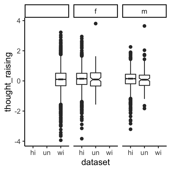
There is basically no variance here. This is an extremely old feature, even though relatively recent work has tied it to a current trend like LOT~THOUGHT merging:
“Irons (2007) found that loss of the upgliding associated with the /O/, or THOUGHT, vowel, a traditional Southern feature, contributed directly to the merger of [THOUGHT] into the LOT vowel in Kentucky.” (Thomas 2020: 530)
Irons, T. L. (2007). “On the status of low back vowels in Kentucky English: More evidence of merger,” Lang. Var. Change 19, 137–180.
PIN~PEN merging
In prenasal environments, the KIT and DRESS vowels can merge in TxE. This is, on one hand, a receding feature.
“Bowie (2000) documented, for a community in Maryland, […] an increase in the differentiation between pre-nasal [KIT] and [DRESS], as in pin and pen, respectively.” (Thomas 2020: 530)
Bowie, D. (2000). “The effect of geographic mobility on the retention of a local dialect,” Ph.D. dissertation, University of Pennsylvania, Philadelphia, PA.
On the other hand it is one of the less encroached-upon features of present-day TxE. Prenasal DRESS nuclei that sound like KIT are fairly frequent in quotidian TxE.
Speaker-level approach
At the speaker level, we can measure the distance between KIT and DRESS in prenasal contexts. Specifically, the Pillai score is of interest here because it provides a more complex, potentially more accurate measure of the distance between two vowel clouds that takes the amount of overlap between them into consideration. Pillai is returned by the R function manova(). See Joey Stanley’s magisterial tutorial on the matter.
Note that Stanley dismisses the significance test that comes with the Pillai score out of the manova() function as “friggin useless” (my summary). So I will use only the Pillai score, and only to produce a ranking of speakers.
The sine qua non citations about Pillai in sociophonetics are:
Hay, Jennifer, Paul Warren & Katie Drager. 2006. Factors influencing speech perception in the context of a merger-in-progress. Journal of Phonetics (Modelling Sociophonetic Variation) 34(4). 458–484. https://doi.org/10.1016/j.wocn.2005.10.001.
They were the first to bring Pillai into sociophonetics.
Hall-Lew, Lauren. 2010. Improved representation of variance in measures of vowel merger. In Proceedings of Meetings on Acoustics (POMA), 1–10. Acoustical Society of America.
She dug Pillai up in the attic of sociophonetics and gave it a new life; argued for its use in studying mergers in several places. Possibly the most frequently cited is:
Nycz, Jennifer & Lauren Hall-Lew. 2013. Best practices in measuring vowel merger. Proceedings of Meetings on Acoustics. Acoustical Society of America 20(1). 060008. https://doi.org/10.1121/1.4894063.
And the original namesake.
Pillai, K. C. S. 1955. Some new test criteria in multivariate analysis. Annals of Mathematical Statistics. Institute of Mathematical Statistics 26(1). 117–121. https://doi.org/10.1214/aoms/1177728599.
speakers <- df_long %>%
  pull(name) %>%
  unique()

pillai_pinpen <- tibble()
for (s in speakers){
  npre <- nrow(pillai_pinpen)
  dat <- df_long %>%
  filter(
    name == s,
    timepoint == 20,
    vowel %in% c("KIT", "DRESS"),
    fol_seg %in% c("M", "N", "NG")) %>%
  mutate(f1_lobanov = as.numeric(f1_lobanov),
         f2_lobanov = as.numeric(f2_lobanov)
  )

  if (length(unique(dat$vowel)) == 2) {
      my_man <- manova(cbind(f1_lobanov, f2_lobanov) ~ vowel, data = dat)
      pil <- summary(my_man)$stats["vowel", "Pillai"]
    }

  if (is.null(pil)) break

  newscore <- tibble(name = s,
                     pinpen_pillai = pil)

  pillai_pinpen <- bind_rows(pillai_pinpen, newscore) %>%
    arrange(pinpen_pillai) %>%
    unique()
}

pillai_pinpen
# A tibble: 53 x 2
   name          pinpen_pillai
   <chr>                 <dbl>
 1 un-1987-aec-f       0.00682
 2 hi-2009-jg-m        0.00888
 3 un-1987-af-m        0.00914
 4 un-1987-afs-m       0.00914
 5 hi-2011-d-m         0.0131
 6 un-1987-bc2-f       0.0162
 7 hi-2010-j-m         0.0253
 8 hi-2011-n-f         0.0295
 9 hi-2010-jr-f        0.0300
10 hi-2010-e-f         0.0326
# … with 43 more rows
Plot these bad boys.
df_long %>%
  group_by(name)                %>%
  slice(1)                      %>%
  left_join(pillai_pinpen)      %>%
  filter(!is.na(pinpen_pillai)) %>%
  #-------------------------------#
  ggplot(aes(x = reorder(name, pinpen_pillai),
             y = pinpen_pillai,
             fill = dataset))    +
  geom_col(stat = "identity",
           width = 0.5)          +
  scale_fill_grey(start = 0,
                  end = 0.8)     +
  coord_flip()                   +
  labs(
    title = "The PIN~PEN merger",
    subtitle = "Some speakers are missing because they lack either PIN or PEN tokens.",
    x = NULL,
    y = "Difference between PIN and PEN (Pillai Index Score)") +
  theme_classic()
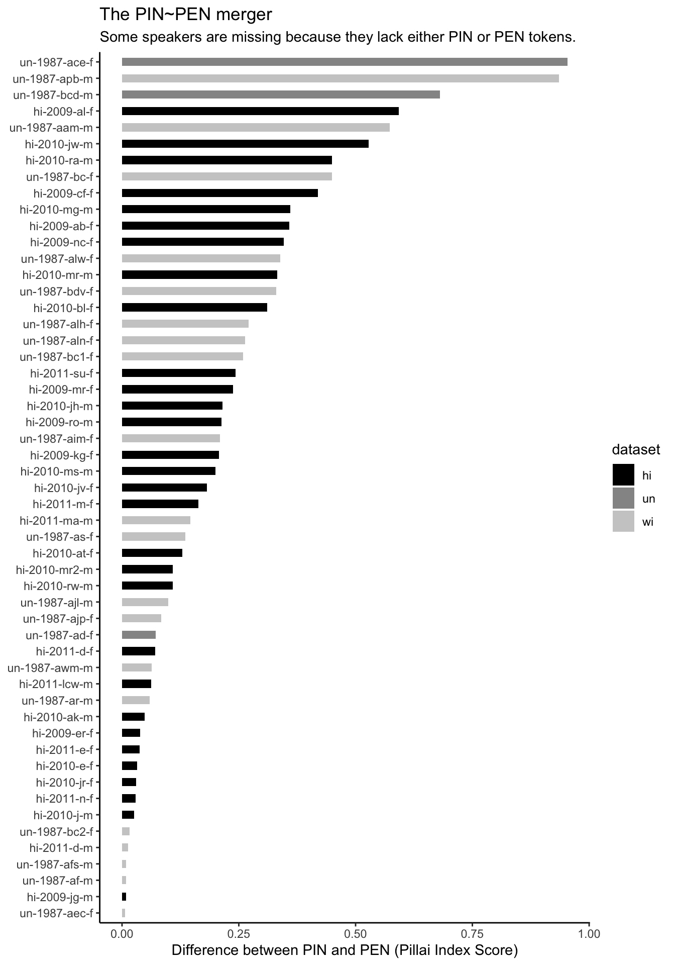
Notice all the hi (i.e. recently interviewed) speakers at the bottom of the plot. Those are the speakers with high degrees of mergers. Which is what I was getting at when I said this feature is not receding.
Token-level approach
speakerPIN <- import("../../_data/data_long_01.RDS") %>%
  filter(vowel %in% c("KIT", "DRESS"),
         fol_seg %in% c("M", "N", "NG")) %>%
  select(name, vowel, timepoint, f1_lobanov, f2_lobanov) %>%
  group_by(name, vowel, timepoint) %>%
  summarise(across(starts_with("f"), mean, .names = "mean_{col}_prenasal"))
df_long <- import("../../_data/data_long_01.RDS") %>%
  left_join(speakerPIN)
We now have a dataset df_long in which for all tokens of KIT and DRESS, the speaker’s average of tokens in prenasal position is given at the far right. For the multivariate analysis, we’ll use tokens of DRESS and measure proximity to KIT.
Below is a comparison of token-level PIN-PEN mergery at 20% and at 50% of vowel duration, when modeled in lmer() with F1(DRESS) as outcome.
mod20 <- lme4::lmer(as.formula(fml),
                    data = dat %>% filter(timepoint == 20))
mod50 <- lme4::lmer(as.formula(fml),
                    data = dat %>% filter(timepoint == 50))

sjPlot::tab_model(mod20, mod50)
| mean f 1 lobanov prenasal | mean f 1 lobanov prenasal | |||||
|---|---|---|---|---|---|---|
| Predictors | Estimates | CI | p | Estimates | CI | p |
| (Intercept) | -4.44 | -7.14 – -1.74 | 0.001 | 3.50 | 0.39 – 6.61 | 0.028 |
| context [internal] | -0.00 | -0.00 – 0.00 | 1.000 | 0.00 | -0.00 – 0.00 | 1.000 |
| dataset [un] | -0.06 | -0.13 – 0.01 | 0.072 | -0.29 | -0.36 – -0.21 | <0.001 |
| gender [m] | 0.01 | -0.03 – 0.05 | 0.567 | -0.07 | -0.11 – -0.03 | 0.001 |
| plt_preseg [liquid] | 0.00 | -0.00 – 0.00 | 1.000 | -0.00 | -0.00 – 0.00 | 1.000 |
| plt_preseg [nasal_labial] | 0.00 | -0.00 – 0.00 | 1.000 | 0.00 | -0.00 – 0.00 | 1.000 |
|
plt_preseg [obstruent_liquid] |
0.00 | -0.00 – 0.00 | 1.000 | 0.00 | -0.00 – 0.00 | 1.000 |
| plt_preseg [oral_apical] | 0.00 | -0.00 – 0.00 | 1.000 | 0.00 | -0.00 – 0.00 | 1.000 |
| plt_preseg [oral_labial] | 0.00 | -0.00 – 0.00 | 1.000 | -0.00 | -0.00 – 0.00 | 1.000 |
| plt_preseg [palatal] | 0.00 | -0.00 – 0.00 | 1.000 | 0.00 | -0.00 – 0.00 | 1.000 |
| plt_preseg [velar] | 0.00 | -0.00 – 0.00 | 1.000 | 0.00 | -0.00 – 0.00 | 1.000 |
| plt_preseg [w/y] | 0.00 | -0.00 – 0.00 | 1.000 | -0.00 | -0.00 – 0.00 | 1.000 |
| plt_folseq [complex_coda] | -0.00 | -0.00 – 0.00 | 1.000 | -0.00 | -0.00 – 0.00 | 1.000 |
|
plt_folseq [complex_one_syl] |
0.00 | -0.00 – 0.00 | 1.000 | 0.00 | -0.00 – 0.00 | 1.000 |
|
plt_folseq [complex_two_syl] |
0.00 | -0.00 – 0.00 | 1.000 | -0.00 | -0.00 – 0.00 | 1.000 |
| plt_folseq [one_fol_syll] | 0.00 | -0.00 – 0.00 | 1.000 | -0.00 | -0.00 – 0.00 | 1.000 |
| plt_folseq [two_fol_syl] | -0.00 | -0.00 – 0.00 | 1.000 | -0.00 | -0.00 – 0.00 | 1.000 |
| yearBorn | 0.00 | 0.00 – 0.00 | 0.002 | -0.00 | -0.00 – -0.00 | 0.035 |
|
ethnicity [african-american] |
-0.27 | -0.33 – -0.22 | <0.001 | -0.38 | -0.44 – -0.32 | <0.001 |
| ethnicity [anglo] | -0.13 | -0.18 – -0.09 | <0.001 | -0.14 | -0.19 – -0.09 | <0.001 |
| Random Effects | ||||||
| σ2 | 0.00 | 0.00 | ||||
| τ00 | 0.01 name | 0.01 name | ||||
| ICC | 1.00 | 1.00 | ||||
| N | 70 name | 70 name | ||||
| Observations | 932 | 932 | ||||
| Marginal R2 / Conditional R2 | 0.734 / 1.000 | 0.732 / 1.000 | ||||
Save data
Save the data sheets. Include suffix _02 in the filename to indicate that this version of the data is produced by the document analysis_02.Rmd.
df_long %>% export("../../_data/data_long_02.RDS")
df_wide %>% export("../../_data/data_wide_02.RDS")