A look at our data
I plan to manually update the 03_alldata_normed.csv in /data regularly. Let’s load it and take a look.
df <- import("../../../data/03_alldata_normed.csv")
df %>% glimpse()
Rows: 457,475
Columns: 30
$ vowelID      <int> 1, 1, 1, 1, 1, 2, 2, 2, 2, 2, 3, 3, 3, 3, 3, 4…
$ name         <chr> "hi-2009-ab-f", "hi-2009-ab-f", "hi-2009-ab-f"…
$ vowel        <chr> "DRESS", "DRESS", "DRESS", "DRESS", "DRESS", "…
$ word         <chr> "YES", "YES", "YES", "YES", "YES", "TWENTY", "…
$ style        <chr> "interview", "interview", "interview", "interv…
$ timepoint    <int> 20, 35, 50, 65, 80, 20, 35, 50, 65, 80, 20, 35…
$ f1_hz        <dbl> 680.5, 1061.8, 810.7, 836.8, 998.3, 656.1, 609…
$ f2_hz        <dbl> 2203.0, 1810.9, 1836.9, 1876.5, 2002.8, 1497.9…
$ f1_lobanov   <dbl> 0.01943932, 2.35367923, 0.81649685, 0.97627566…
$ f2_lobanov   <dbl> 1.1975892, 0.1243169, 0.1954852, 0.3038799, 0.…
$ dur          <dbl> 0.23, 0.23, 0.23, 0.23, 0.23, 0.17, 0.17, 0.17…
$ plt_vclass   <chr> "e", "e", "e", "e", "e", "e", "e", "e", "e", "…
$ plt_manner   <chr> "fricative", "fricative", "fricative", "fricat…
$ plt_place    <chr> "apical", "apical", "apical", "apical", "apica…
$ plt_voice    <chr> "voiceless", "voiceless", "voiceless", "voicel…
$ plt_preseg   <chr> "w/y", "w/y", "w/y", "w/y", "w/y", "w/y", "w/y…
$ plt_folseq   <chr> "", "", "", "", "", "complex_one_syl", "comple…
$ pre_seg      <chr> "Y", "Y", "Y", "Y", "Y", "W", "W", "W", "W", "…
$ fol_seg      <chr> "S", "S", "S", "S", "S", "N", "N", "N", "N", "…
$ context      <chr> "internal", "internal", "internal", "internal"…
$ dataset      <chr> "hi", "hi", "hi", "hi", "hi", "hi", "hi", "hi"…
$ yearRecorded <int> 2009, 2009, 2009, 2009, 2009, 2009, 2009, 2009…
$ initials     <chr> "ab", "ab", "ab", "ab", "ab", "ab", "ab", "ab"…
$ gender       <chr> "f", "f", "f", "f", "f", "f", "f", "f", "f", "…
$ yearBorn     <int> 1983, 1983, 1983, 1983, 1983, 1983, 1983, 1983…
$ ethnicity    <chr> "anglo", "anglo", "anglo", "anglo", "anglo", "…
$ townRaised   <chr> "austin", "austin", "austin", "austin", "austi…
$ occupation   <chr> "", "", "", "", "", "", "", "", "", "", "", ""…
$ beg          <dbl> 8.779, 8.779, 8.779, 8.779, 8.779, 13.496, 13.…
$ fileName     <chr> "../../../04 formant measurements (5 points DA…
Time depth
df$dataset <- ifelse(df$dataset == "", "wi", df$dataset)

df %>%
  tabyl(dataset) %>%
  select(1, 2)
 dataset      n
      hi 194170
      un  19420
      wi 243885
A wide-format version of the data, with one row per unique vowel token
df_wide <- df         %>%
    pivot_wider(names_from = timepoint,
                values_from = c(f1_hz, f2_hz, f1_lobanov, f2_lobanov))
Define phonetic variables
We may need to come at our df from two sides:
- token-level variation
- speaker-level variation
We will see how consistently we’ll do the latter; certainly the place to start is the prior. However, before we can do token-level moves we still need some utility purpose functions, which are in many cases speaker-level.
Let us go through our list of diagnostic features and define functions to describe each of them.
Utility functions
Get mean for vowel for speaker
Define a function that takes a dataset, speaker and vowel as arguments and returns the centroid in the form of a numeric vector. The function will be called getspeakervowel().
# moved to functiondefs.R
Let us try this out with un-1987-bcd-m as speaker and FLEECE as vowel.
df %>% getspeakervowel("un-1987-bcd-m", "FLEECE")
$f1lob
[1] -1.320854

$f2lob
[1] 0.08258948
Given this output, we could now use as.numeric() to turn this output into a vector, or as_tibble() to turn it into a tibble, i.e. dataframe.
Get vowel space centroid for speaker
To calculate the vowel space centroid for a speaker, we use their F1/F2 for the four corner vowels and average them. I have run this by a couple of full-time phoneticians and they gave it a pass (i.e. “thumbs up”). Name of this function: getcentroid().
# moved to functiondefs.R
Let’s try this out with un-1987-bcd-m as speaker.
df %>% getcentroid("un-1987-bcd-m")
$f1lob
[1] -0.7226548

$f2lob
[1] 0.03302487
Seems to be working. As before: given this output, we can now use as.numeric() to turn this output into a vector, or as_tibble() to turn it into a tibble, i.e. dataframe.
Get Cartesian distance between two vowels
First, define a general function for calculating distance between two sets of x-y-coordinates. This will be helpful because it allows working with individual tokens as well as centroids without having to repeat the distance formula. Name of this function: cdis().
# moved to functiondefs.R
The next function, getCD1(), expects to be given two vowels (in the form of numeric vectors) and returns the Cartesian Distance.
# moved to functiondefs.R
Get Cartesian distance between vowel centroids for speaker
“Cartesian Distance”, as I understand it, is a version of Euclidian Distance, specifically in 2-D space. Name of this function: getCD2().
Note the use of the nth() function to extract items from numeric vector.
# moved to functiondefs.R
Let’s try this out with
dfas data,un-1987-bcd-mas speaker,- KIT as vowel 1, and
- TRAP/BATH as vowel 2.
df %>% getCD2("un-1987-bcd-m", "KIT", "TRAP/BATH")
[1] 0.392647Seems to be working.
Add trajectory length for all vowels to the wide dataframe
Trajectory length is the sum of euclidean distances n F1/F2 space between equidistant timepoints during vowel articulation. Olsen et al. (2017) use 20-35-50-65-80, i.e. the same output that we have from DARLA. Trajectory length was initially included to model PRICE/PRIZE glide weakening, but it is a meaninful variable for all vowels and will be of interest when looking at any monophthong undergoing diphthongization and any diphthong undergoing monopthongization, so it makes sense to just calculate this for the whole dataset.
First, a function that calculates trajectory length based on five sets of f1/f2 coords. Name of this function: getTL().
# moved to functiondefs.R
Ok, and now we apply this to every row of the wide dataframe with purrr::pmap_dbl (because rowwise() is no longer recommended).
Let’s visualize how the different vowels do in terms of trajectory length in the data on the whole
ggplot(data=df_wide) +
  geom_boxplot(aes(x=vowel,y=trajLN)) +
  theme_classic() +
  theme(axis.text.x = element_text(angle = 30))
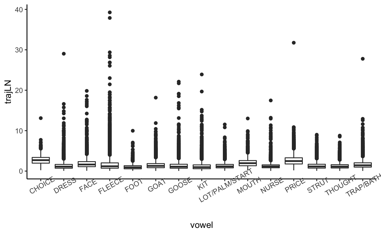
Looks good. The diphthongs show higher median trajectory lengths, as expected, followed by the tense vowels which are more likely to have some degree of diphthongization (and are simply longer), although there isn’t much of a difference between tense and lax vowels. FLEECE is interesting because lots of outliers with very long trajectory. Suggests non-uniformity in speaker behavior, with some doing a more diphthongal realization than the majority.
Also note that all of these distributions are heavily skewed. When working with trajectory lengths under assumptions of normality, we’ll need to apply appropriate transformations.
Add onset-glide (20-80) height difference to all vowels in the wide dataframe
Just how much the tongue raises/lowers in the glide compared to the onset. This may be more relevant than trajectory length in cases where the focus is more specifically on the big picture of glide raising/lowering.
df_wide <- df_wide %>%
  mutate(glideRaise = f1_lobanov_20 - f1_lobanov_80)
Plot to make sure it makes sense:
ggplot(data=df_wide) +
  geom_boxplot(aes(x=vowel,y=glideRaise)) +
  theme_classic() +
  theme(axis.text.x = element_text(angle = 30))
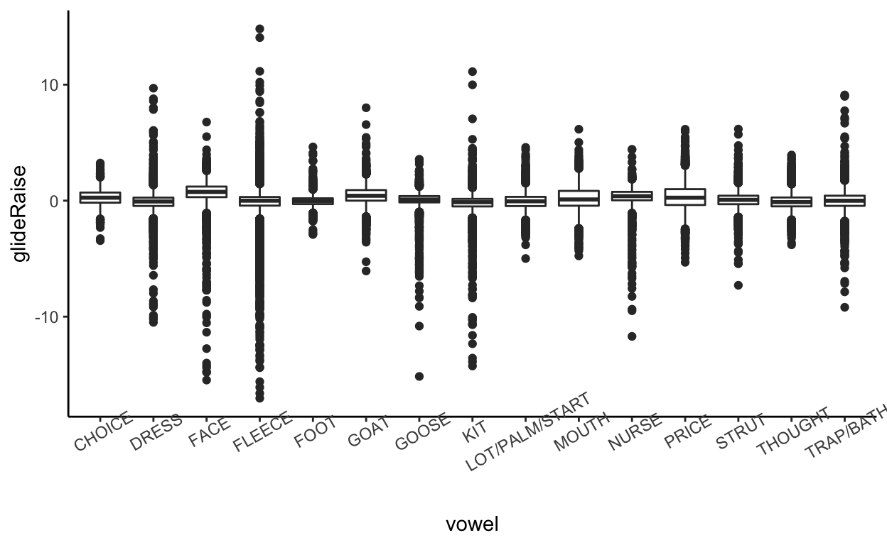
Makes sense in terms of general directions, but holy shit is there a lot of variance! Is this normal when working with phonetic data (because duration and coarticulation effects are not controlled for, etc.)?
Add onset-glide (20-80) frontness difference to all vowels in the wide dataframe
How much the tongue fronts/retractss in the glide compared to the onset. Again, this may be more relevant than trajectory length in cases where the focus is more specifically on the big picture of glide fronting/retraction.
df_wide <- df_wide %>%
  mutate(glideFront = f2_lobanov_80 - f2_lobanov_20)
Plot to make sure it makes sense:
ggplot(data=df_wide) +
  geom_boxplot(aes(x=vowel,y=glideFront)) +
  labs(x="") +
  theme_classic() +
  theme(axis.text.x = element_text(angle = 30))
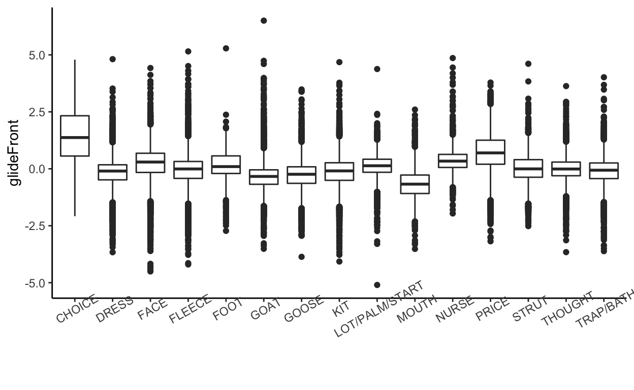
Looks good.
Add onset-glide (20-80) euclidean distance to all vowels in the wide dataframe
A pretty standard measure for looking at diphthongs. Fox and Jacewicz (2009) refer to this as “vector length”.
Plot to make sure it makes sense:
ggplot(data=df_wide) +
  geom_boxplot(aes(x=vowel,y=dist2080)) +
  theme_classic() +
  theme(axis.text.x = element_text(angle = 30))
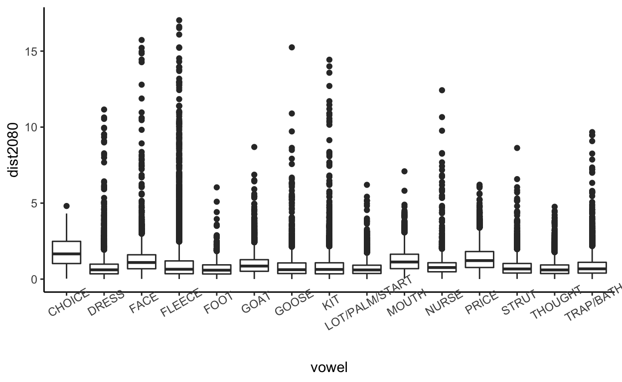
Looks good as well.
Add spectral rate of change to the wide dataframe
“Fox and Jacewicz incorporate an additional measure, spectral rate of change, to calculate how fast spectral change occurs across the vowel’s duration, by dividing the trajectory length by the duration.” (Farrington et al. 2018: 192) Seems like the concept is pretty hazy and of a “perhaps there’s something there” nature, but we have to actually check Fox & Jacewicz (2009), which seems an important paper anyway.
df_wide <- df_wide %>%
  mutate(spectralRate = trajLN/dur)
Plot to make sure it makes sense:
ggplot(data=df_wide) +
  geom_boxplot(aes(x=vowel,y=spectralRate)) +
  theme_classic() +
  theme(axis.text.x = element_text(angle = 30))
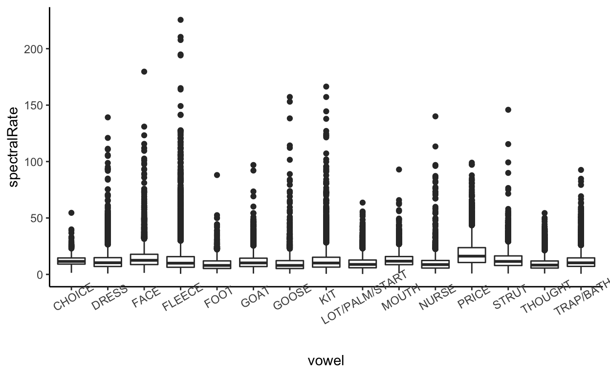
Difficult to evaluate, because I am not sure what to expect. Interesting in any case that PRICE has the highest median spectral change, given glide weakening in traditional Southern US English.
Save data
We now have two versions of the data going. Let’s save them at the end of this sheet in order to make them available for work in the next sheet. Let’s use RDS format for ease of use. Include the suffix _01 in the filename to indicate that this version of the data is produced by the document analysis_01.Rmd.
df %>% export("../../_data/data_long_01.RDS")
df_wide %>% export("../../_data/data_wide_01.RDS")
Feature coding functions
Generally, work on each feature from here on down should
- prefer to form an index,
- form a new column where appropriate, but that column should contain values only in rows where it’s plausible and NAs otherwise;
- draw on the utility functions above wherever possible.